On this page, you should find all the information about exercises of the Digital Image Processing course.
Evaluation - how can you earn a credit
During the exercises, we will cover some topic of digital image processing. Your task is complete them and handover them for final grading.
| Task | Points |
| Convolution | 2 |
| Anisotropic diffusion | 4 |
| Discrete Fourier Transform | 4 |
| Inverse Discrete Fourier Transform | 3 |
| Filtering in frequency domain | 4 |
| Lens distortion removal | 4 |
| Histogram equalization | 2 |
| Projective transform | 5 |
| Edge detection | 2 |
| Edge thinning | 3 |
| Double thresholding | 4 |
| Backprojection | 3 |
Other sources
A simple tutorial describing how to program with the OpenCV is provided in the following link: Introduction to OpenCV
Exercise 1
You can use a project for the Visual Studio 2017 in the Windows environment to code the exercise.
You can use a project for the Visual Studio Code in the Linux environment to code the exercise.
First, install these two VSCode extensions:
        code --install-extension ms-vscode.cpptools
        code --install-extension ms-vscode.cmake-tools
You can find a color image of Lena that we can use for our experiments. It's included in our project.
You can also read explanatory text that describes the first exercise in detail. Basic operations with images are described.
Grayscale image Moon that we can use for our experiments with Gamma correction and contrast enhancement.
Exercise 2
We'll implement a convolution algorithm. You can apply Box blur, Gaussian blur, Laplace, or other matrices as a convolution mask.
Exercise 3
Filtering using anisotropic diffusion (see instructions).
Exercise 4
In this exercise, we will compute the Discrete Fourier Transform (EN, CZ) and also Inverse Discrete Fourier Transform (EN).
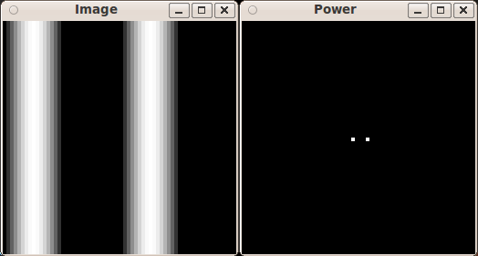
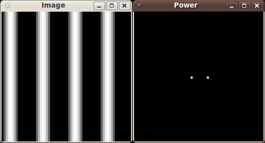
Images below show the output for two different sin waves.
The first is with period 4, the second with period 8.
You can clearly see the frequency of the sin wave in the output frequency spectrum.


We can use earth.png and lena64.png grayscale images for our experiments with the DFT and IDFT (they are 64x64 px, so our O(n^4) algorithm doesn't have to chew too much data).
Exercise 5
In this exercise, we'll apply low and high pass filters in the frequency domain. We can try to remove a noise, bars, etc. Follow the text (EN, CZ) to complete the exercise.
Here are a few images, that we can use for our experiments: lena64.png, lena64_noise.png, lena64_noise2.png, lena64_bars.png.
Exercise 6
In this exercise, we'll implement a simple removal of a geometric distortion. Description of the algorithm is provided in this text.
The following images can be used for our experiments: Panorama, Window.
A simple template program is provided.
Exercise 7
Image for histogram equalisation: uneq.jpg
You can see how it should look like in the screenshot.
Instructions how to implement histogram equalization.
Exercise 8
We'll have fun with the projective transform. Use the image of our university and the Czech flag as input images. The result should look like: this.
Use this text that describes the projective transform.
Exercise 9
Color image of a valve (already available in the provided project) that we can use for our experiments.
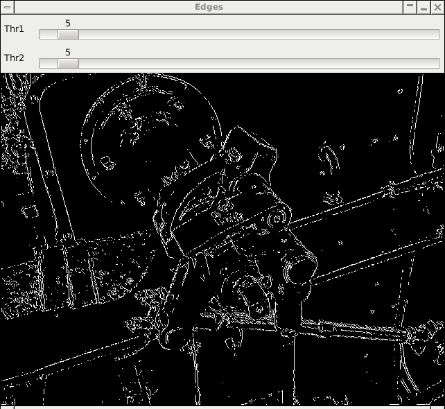
We'll implement x and y derivatives of image (see Sobel operator) and visualize edge magnitudes of the valve image:
Also, implement edge thinning on the valve image:

Exercise 10
We'll implement double thresholding on the valve image:

Exercise 11
We'll implement the backprojection algorithm.
Exercise 12
Exercise 13
Final evaluation of tasks.

