Edge Detection

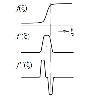
Image segmentation is an important task in image analysis. This process extracts objects from an image background. Since the objects often consists of another color (brightness) than the background, the image segmentation is usually based on the detection of object boundaries. These boundaries contains edges - a location in the image where the color (brightness) function significantly changes. Therefore, the location of edge can be determined using the derivative of the function (see Figure fig:edges). In this exercise, you will implement two basic edge detection methods.

First Derivative

As it is seen in Figure fig:edges, the absolute value of first derivative is high at the image point where the edge is located. Therefore, the edge is determined using derivatives \(\partial f / \partial x\) and \(\partial f / \partial y\) describing changes in the brightness function in the \(x\) and \(y\) directions. Practically, we work with the images in the discrete form, therefore, the derivatives are substituted by the differences

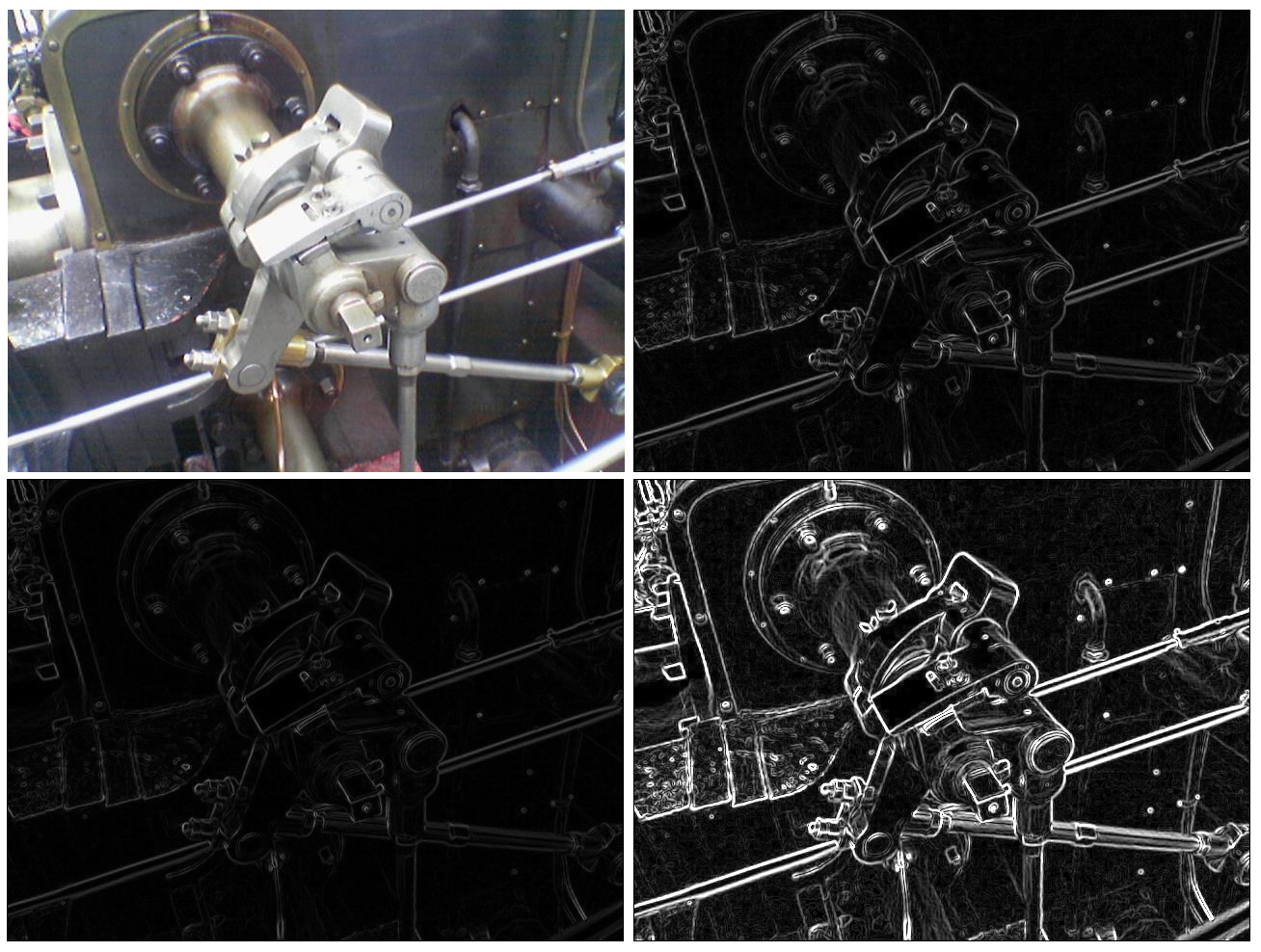
\[\begin{eqnarray} f_x(x,y) = f(x+1, y) - f(x,y)\\ f_y(x,y) = f(x, y+1) - f(x,y) \end{eqnarray}\] The size of edge is computed as \[\begin{equation} e(x,y) = \sqrt{f^2_x(x,y) + f^2_y(x,y)}. \end{equation}\] This value is computed for all image pixels. If \(e(x,y)\) is higher than a chosen threshold, it is considered as a real edge. The result of this method (in the normalized form) can be seen in Figure fig:result.

Second Derivative

In Figure fig:edges, it is shown that the edge can be detected using second derivate. The brightness function reaches the positive and negative extrema, the zero value between these two extrema determines the edge. For this purpose, the Laplacian operator can be used. Similarly as before, the brightness function is analyzed in the \(x\) and \(y\) directions, i.e. \(f_{xx}=\partial^2f(x,y) / \partial x^2\), \(f_{yy}=\partial^2f(x,y) / \partial y^2\). The Laplacian operator is defined as \[\begin{equation} \triangledown^2 f(x,y) = f_{xx}(x,y)+f_{yy}(x,y). \end{equation}\] Similarly as before, due to the discrete image domain, the derivatives are replaced by the differences in the form \[\begin{eqnarray} f_{xx}(x,y) = f(x-1, y) - 2f(x,y)+f(x+1,y)\\ f_{yy}(x,y) = f(x, y-1) - 2f(x,y)+f(x,y+1). \end{eqnarray}\] Using the Laplacian operator, the equation is in the form \[\begin{equation} \triangledown^2 f(x,y) = f(x-1, y)+f(x+1,y)+f(x, y-1)+f(x,y+1)-4f(x,y). \end{equation}\] The result of this method (in the normalized form) can be seen in Figure fig:result.

Sobel Operator

This operator is also based on the differences between the pixel values in the \(x\) and \(y\) directions. For computing the size of edge at \((x,y)\), the Sobel operator uses values of all the neighboring pixels. Let us use the labels of the neighboring pixels as it is shown in Figure fig:labeling.

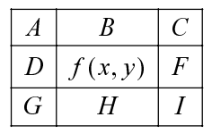
The value of \(f(x,y)\) is computed as \[\begin{eqnarray} f_x(x,y)=(C-A) + 2(F-D) + (I-G)\\ f_y(x,y)=(A-G) + 2(B-H) + (C-I) \end{eqnarray}\]

These formulas can be represented as \(3\times 3\) convolution masks as it is shown in Figure fig:sobel_masks. Therefore, you can compute the output image using image convolution. The result of the Sobel operator can be seen in Figure fig:result.